Teaching a Computer to Tell Walking from Running

Watch what happens when you take 250 frames of someone waving their arms and compress them into a single grayscale image where bright means just-now and dim means a moment ago.

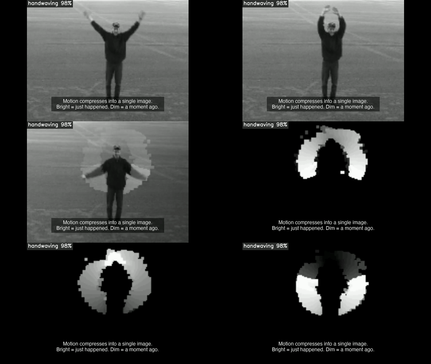Handwaving as raw video, then the same motion compressed into a single Motion History Image. Bright pixels mark where motion just happened; dim pixels mark where it happened a moment ago.

That’s a Motion History Image. The lobed shape with the bright recent ring and the dim older fringe is the temporal signature of arm-waving, sitting still in two dimensions. The whole arc of motion across ten seconds, collapsed into a single picture.

This is the question I wanted to answer: is this representation, plus a random forest, plus some careful feature engineering, enough to get classical computer vision to 86% accuracy on a six-action benchmark? It turns out, yes, but the path there matters more than the headline number. Most of the work was not in tuning the classifier. It was in reading the model’s per-class explanations and using them to figure out which features it actually needed.

Why classical computer vision, in 2026

The benchmark is the KTH Human Actions dataset: 599 video clips of 25 people each performing six actions (walking, jogging, running, boxing, handwaving, handclapping) outdoors and indoors at three different scales. The dataset is from 2004, which makes it old enough to predate every deep learning paper you have read. People still use it as a sanity check for new methods, but the modern leaderboard is dominated by 3D CNNs and transformers that need GPUs to train.

This project does none of that. The pipeline is end-to-end classical: motion masks from frame differencing, motion history images, Hu invariant moments, a random forest. No neural network, no GPU. The reason is not nostalgia. It is that explicit features make explainability tractable in a way that learned representations do not. When I want to know why my model thinks one clip is jogging and another is walking, I can read the per-feature SHAP attribution and see exactly which feature pushed the prediction which way. With a 3D CNN, I can see saliency maps; that is not the same thing.

I built this as the final project for a graduate computer vision course while operating BizziB AI, a data and AI consultancy. The throughline of both is a question I keep coming back to: how do we measure human movement accurately and explainably? My parallel project on the Bayesian side wearable-calibration-bayes attacks the same question from the IMU sensor side, asking whether step-counting algorithms produce systematically biased cadence estimates across body geometry. This project attacks it from the video side. Both lean on classical statistics and explicit features rather than learned representations, because for movement measurement, knowing why a model thinks what it thinks matters as much as the headline accuracy.

The pipeline at a glance

The pipeline has seven stages, and each one earns its place by doing exactly one thing.

Stage 1: motion mask. Take two consecutive grayscale frames. Subtract them, threshold the difference at some theta, and you get a binary image showing where motion happened. KTH at 25 fps produces an edge-like one-or-two-pixel ghost outline at the boundaries of the moving subject, which a simple morphological open destroys. Closing first bridges the ghost gap, then opening removes residual specks. That sequence (close-then-open) was the locked choice after the boxing clips revealed the failure mode of open-only.

**Stage 2: MHI accumulation. **A binary motion mask tells you where motion is happening at one instant. The shape of motion over time is what distinguishes walking from waving. The MHI gives each pixel a freshness counter: when the pixel is in motion at the current frame, set its counter to a maximum value tau. When it is not in motion, decrement the counter by 1, never below 0. After many frames, the resulting image shows bright pixels where motion just happened and dim pixels where it happened a moment ago. The right tau depends on how long the action takes; walking is slow and deserves a longer memory than handclapping. I locked a per-action tau from a coarse-then-refined sweep over each of the six actions.

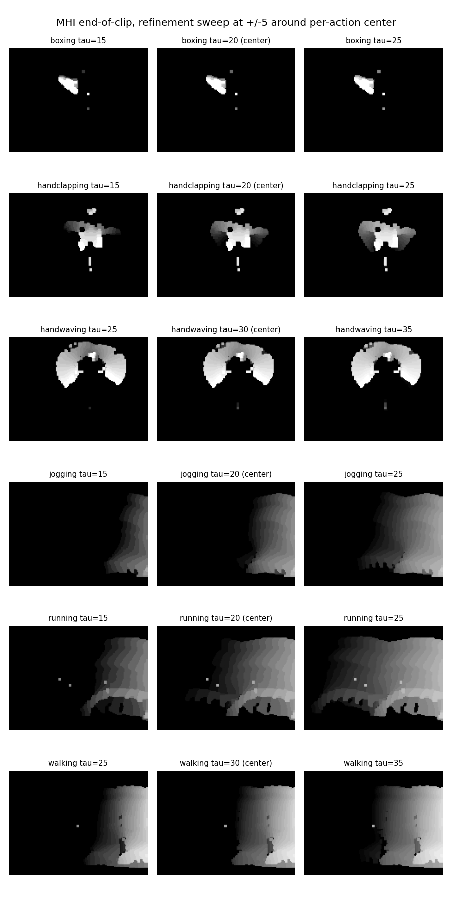Refined per-action τ sweep at 5-frame resolution. The locked τ values are the ones that produce stable MHI coverage without saturating the frame. Walking and jogging get longer memory; handclapping gets the shortest.

Stage 3: image moments and Hu invariants. This is where shape descriptors enter. Image moments are weighted sums of pixel intensities times powers of pixel coordinates. Raw moments depend on where the shape sits in the frame; central moments shift to the centroid; normalized central moments scale away the size; Hu’s seven invariants combine those normalized moments into quantities that survive translation, scale, and rotation. The course banned cv2.HuMoments, which was probably the right call because writing them out from the definitions makes the meaning of each invariant much clearer than calling a black-box function. I used a sign-preserving log transform on the Hu values because the raw magnitudes span many orders of magnitude.

Stage 4: multi-channel feature stacking. This is the architectural choice that earns its own section.

Stage 5: random forest classifier. Tuned via subject-grouped leave-one-subject-out cross-validation against the training half. I benchmarked random forest, histogram gradient boosting, and gradient boosting; random forest won, and the cross-model spread within 0.024 told me the ceiling was feature-driven, not model-driven.

Stage 6: evaluation. A held-out 9-subject split (the test subjects never appear in training) plus a confusion matrix, per-class accuracy, and an n_estimators error sweep.

Stage 7: annotation. Run the full pipeline on a clip and overlay the predicted action and confidence on every frame, like the labels you saw in the opening video.

Multi-channel stacking is the central architectural call

The standard pipeline picks one theta (the binary threshold) and one kernel size (the morphology kernel) and runs everything downstream from that single choice. The problem is that different actions look best at different settings. Boxing has localized, low-amplitude motion at the chest, which needs a low theta to even register; walking has whole-body translation that survives a higher theta cleanly. There is no single setting that is best for all six actions.

Instead of picking one, I ran the motion mask, MHI, and moments stages once per channel for an explicit list of (theta, kernel) combinations and concatenated the per-channel moment vectors into a single feature row. Eight channels, seven log-Hu invariants per channel, 56 features in the v1 baseline. I do not know which (theta, kernel) is best for handwaving versus walking. The random forest does, because it sees all eight at once and learns per-action-pair channel importance from the data.

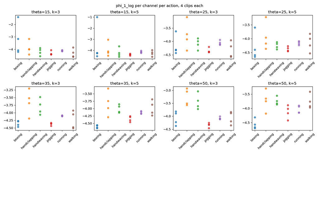The first Hu invariant (log φ₁, a global shape descriptor) per action across all 599 KTH clips, broken out by channel. Low-θ panels (left) show long tails: a few clips’ motion masks fragment at the lowest threshold and produce extreme outliers. At θ ≥ 25 the masks consolidate and the per-action distributions tighten. No single panel separates all six actions cleanly.

You can see in the per-channel phi_1_log panels that no single panel separates all six actions cleanly. Each channel exposes different distinctions. Boxing has an outlier subject at the lowest theta because that subject’s motion masks fragment at the threshold; the outlier disappears at theta >= 25 where the masks consolidate. The random forest can draw on whichever channel is reliable for any given decision.

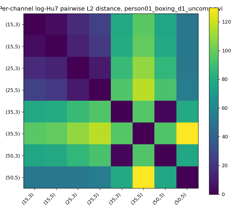Per-channel log-Hu pairwise L2-distance heatmap on a single clip. The block structure splits low-θ channels from high-θ channels, confirming the eight channels carry genuinely different information rather than redundant copies of each other.

The pairwise distances between channels (computed on the same single clip) confirm that the eight channels carry genuinely different information rather than redundant copies. The block structure splits low-theta channels from high-theta channels, exactly the kind of diversity you want a stacking grid to capture.

This decision turns out to matter for the SHAP analysis later, because per-channel attribution gives a granular view of which channels carried which actions. We will get to that.

The 56-feature baseline lands at 70%, and the diagnosis matters more than the number

Trained on the multi-channel Hu-only feature matrix, the tuned random forest reaches 0.7037 test accuracy. Histogram gradient boosting at 0.6764 and gradient boosting at 0.6839 sit within 0.024 of that number. Three independently tuned ensemble families tied within 2.4 percentage points means the ceiling is not the choice of classifier; it is the choice of features.

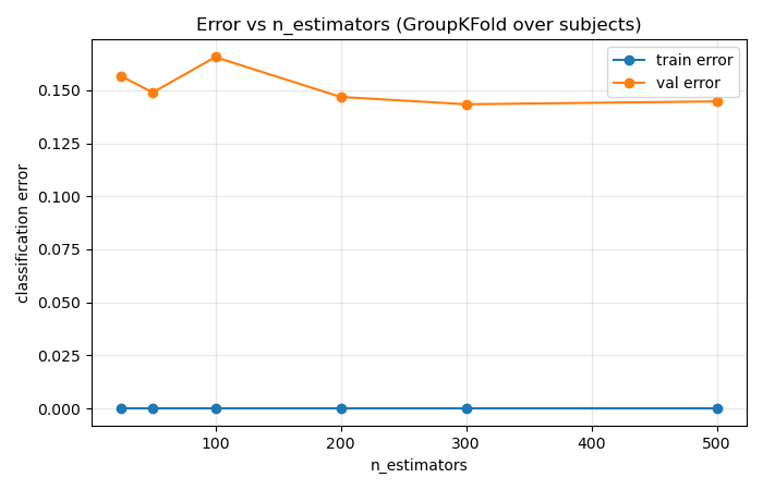Train and validation classification error rate as a function of n_estimators on the v1 baseline (56 features). Training error drops to zero by 100 trees while validation error plateaus around 0.15. More trees do not help; the bottleneck is the feature space, not the classifier capacity.

The validation error curve confirms the diagnosis. By 200 trees, the validation error has plateaued and adding more trees does nothing. The model has extracted everything the feature space contains and is leaving accuracy on the table because the feature space itself is incomplete.

The next step is therefore feature engineering, not more classifier tuning. The question becomes: which features should I add? This is where SHAP earns its place.

SHAP as a feature-engineering compass

TreeSHAP gives you a per-feature signed attribution for every prediction. Sum across samples within a class and you get a per-class signature: which features push toward this class, which features push away, and how strongly. Most SHAP write-ups present this as “here is what my model learned.” I read it as a deficit map.

A class that has strong positive SHAP on a few features that genuinely capture its motion structure is well-served by those features. A class that has weak attribution everywhere is being predicted by elimination. A class that has negative aggregate attribution on the features it shares with other classes is being actively confused with them. Each pattern points at a different kind of fix.

The v1 SHAP analysis on the Hu-only baseline surfaced three specific deficits, each pointing at a different feature family.

Deficit 1: Boxing was being actively confused with the other arm classes

Hu invariants are scale-invariant by design. They throw away absolute size, which is a feature, not a bug, when you want shape descriptors that survive zoom and distance. But it means the Hu features cannot distinguish actions by how much motion is happening. Boxing produces small, dense motion regions; running produces large, elongated ones. Hu cannot see that.

The v1 SHAP showed boxing with signed-negative aggregate attribution, meaning the Hu features were not just unhelpful for boxing, they were pushing predictions away from boxing toward the other arm classes. Adding scalar shape and mass features (bounding box aspect ratio, log of m_00 which is the total motion mass, mean intensity over nonzero pixels, and nonzero pixel count) gave the classifier orthogonal handles. Boxing’s per-class accuracy lifted from 0.58 to 0.81, the largest single gain. Test accuracy went from 0.7037 to 0.8333.

Deficit 2: Upper-body actions and full-body actions used the same global descriptors

Hu invariants on the full silhouette capture global shape but blur the vertical structure that distinguishes upper-body actions (handclapping, handwaving, the arm component of boxing) from full-body actions (walking, jogging, running). I added half-silhouette Hu invariants: seven log-Hu values on the top half of the MHI plus seven on the bottom half. The intuition I started with was that the upper-vs-lower mass ratio would do the work. The intuition I ended with, after the SHAP told me what was actually happening, was that the shape of motion within each half mattered more than the relative mass between them. Either way, the discriminative signal was real. Test accuracy went from 0.8333 to 0.8519.

Deficit 3: Walking, jogging, and running share a silhouette structure

The locomotion three differ primarily in cadence. Hu invariants and scalar mass features capture spatial structure but average out temporal variation. To capture cadence directly, I took a five-bin FFT of the per-frame motion-mask area time series. The first few magnitude bins capture gait frequency, which is the cleanest signal for distinguishing walking from jogging from running.

This was the closing addition. Test accuracy went from 0.8519 to 0.8611. The lift concentrated on the locomotion classes exactly as the periodicity hypothesis predicted.

The progression as a table:

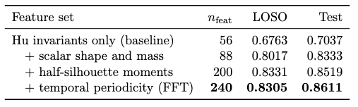Each row adds one feature family on top of the row above. The bundle+p5+p6 row at 240 features ships as the final model, lifting test accuracy from 0.7037 to 0.8611 across three SHAP-driven additions.

Each row adds one feature family on top of the row above. Each addition was identified from the SHAP surface of the previous model, designed to close a specific deficit, and validated against test accuracy as a separate gate.

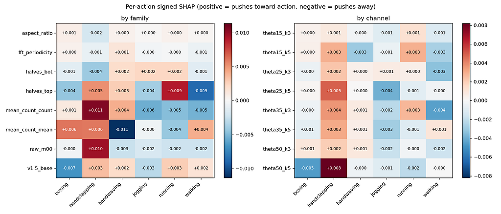Per-class signed TreeSHAP attribution on the final 240-feature random forest. Red pushes toward the class, blue pushes away. The mass and intensity rows light red for boxing and walking; the nonzero-count row lights red for handclapping and handwaving with opposite signs (the arm-action duality). Top-half log-Hu dominates running. Jogging is conspicuously dim across families; the model has no confident positive signal for jogging, which is why it gets predicted by elimination.

The final model’s SHAP surface, broken out by feature family on the left and by channel on the right, makes the architecture visible. Mass and intensity rows light red for boxing and walking. The nonzero-count row lights red for handclapping and handwaving with opposite signs (the arm-action duality). Top-half log-Hu dominates running. Jogging is conspicuously dim across families: the model has no confident positive signal for jogging, which is why it gets predicted by elimination. Park that observation; it is going to matter for the failure modes.

Where the model is wrong, it is mostly unsure

The headline test accuracy is 0.8611. Multi-seed mean across 8 random seeds is 0.8640 with a standard deviation of 0.0078, range 0.8519 to 0.8750. The result is stable.

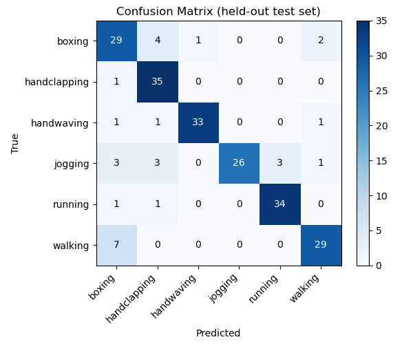Held-out test confusion matrix on 215 clips, 36 per action class. Diagonal cells are correct predictions. The two off-diagonal clusters: jogging confused with walking and running (cadence-adjacent locomotion), and boxing confused with handclapping (arm-action duality). Every other off-diagonal cell is at most a single-digit count.

The confusion matrix on 215 held-out test clips shows two clusters of confusion: jogging-as-walking and jogging-as-running (cadence-adjacent locomotion), and handclapping-vs-boxing (arm-action duality). Every other off-diagonal cell is at most a single-digit count. Jogging is the per-class accuracy floor at 0.722, predicted as walking three times and running three times.

What I find interesting is not that the model fails at these two boundaries (anyone who has watched the clips would expect this) but how it fails. Of the most-confidently-wrong test clips per action, none has confidence above 0.65. Every failure is a “model is unsure” beat, not a “model is confidently wrong” beat. The failures are at class boundaries where the categories themselves are genuinely close, not deep inside class distributions where the model has misunderstood something fundamental.

Failure mode 1: cadence-adjacent locomotion

Here is the most-confidently-wrong jogging clip. The model predicted walking at 59% confidence.

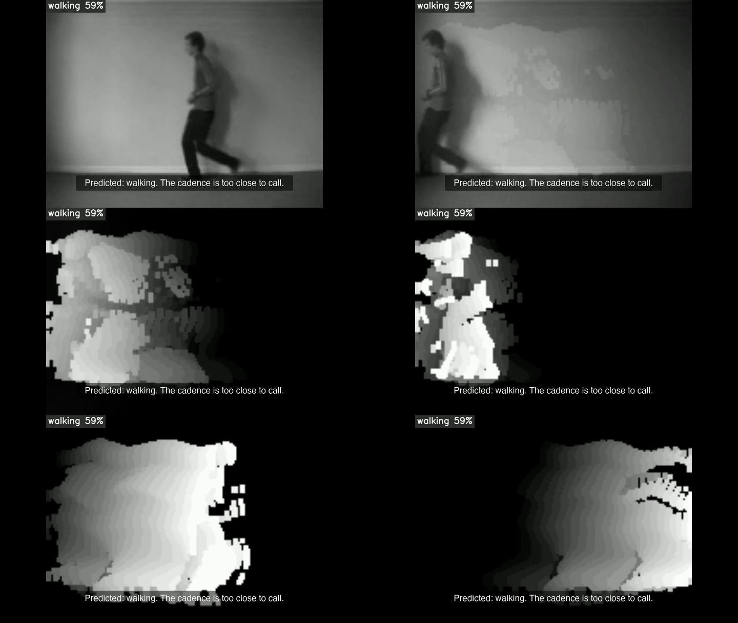A jogging clip the model predicted as walking at 59% confidence. The MHI variant shows the leg-trajectory arc that was indistinguishable from walking’s signature.

You can see why. The cadence is at the boundary between walking and jogging, the silhouette structure is identical, and the leg trajectories trace the same arc shape in the MHI. The model is not wrong because it failed to see something. It is wrong because the categories themselves overlap at this speed.

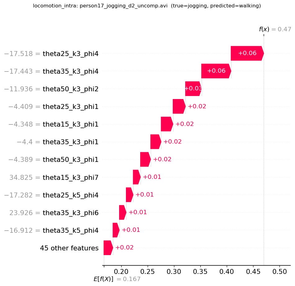SHAP waterfall on the most-confidently-wrong jogging clip (predicted: walking at 59% confidence). Per-feature attribution shows the FFT periodicity bins pushing the prediction toward walking. The feature engineering worked exactly as designed; on this specific clip the cadence resembles walking more than jogging.

The SHAP waterfall on this specific failure clip shows the per-feature attribution toward the wrongly-predicted class (walking). The dominant push toward walking comes from the FFT periodicity bins that I had added specifically to discriminate locomotion. The feature engineering worked exactly as designed; it pushed the prediction toward whichever locomotion class the cadence most resembled. On this clip the cadence resembles walking. The model is right to be uncertain at this boundary; a human watching the same clip and not told the ground truth would be uncertain too.

Failure mode 2: arm-action duality

Here is the most-confidently-wrong boxing clip. The model predicted handclapping at 60% confidence.

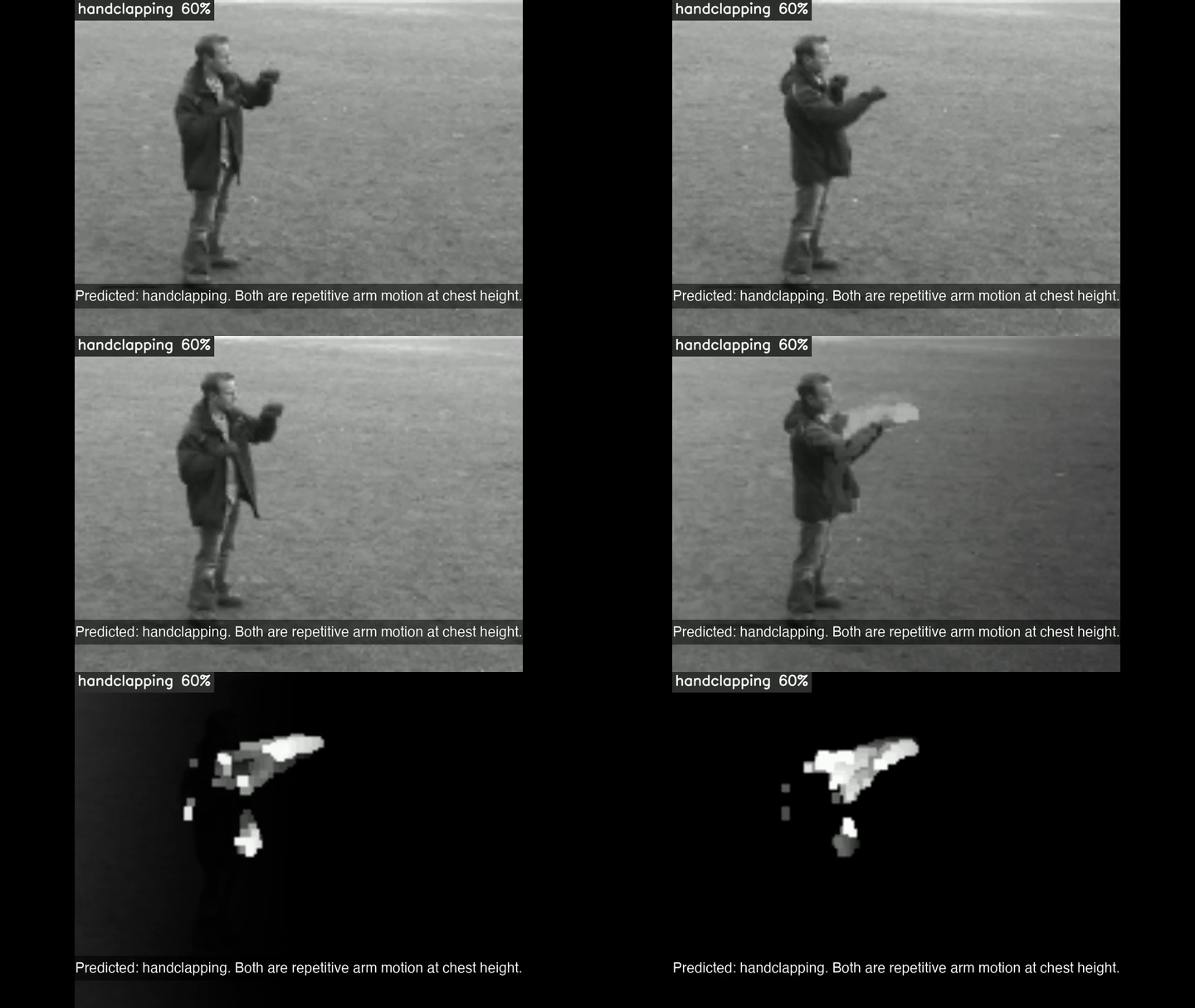A boxing clip the model predicted as handclapping at 60% confidence. Both actions produce repetitive arm motion at chest height, visible in the MHI as a horizontal band.

Boxing and handclapping are both repetitive arm motions at chest height. The MHI for both produces a horizontal band of motion concentrated near the upper-middle of the frame, with bright recent strikes and dim older ones. The visual signature differs in subtle ways (boxing has more vertical extent because the punch travels forward and back, handclapping is more compact and horizontal) but the difference is small enough that a low-confidence prediction is reasonable.

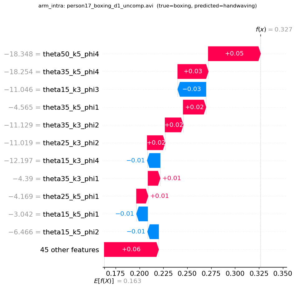SHAP waterfall on the most-confidently-wrong boxing clip (predicted: handclapping at 60% confidence). The model leans on the same feature families it uses for both classes (nonzero count, halves_top) with sign-flipped weighting. The arm-action duality shows up directly in the attribution.

The SHAP attribution on this failure shows the model leaning on the same feature families it uses for both classes (nonzero count, halves_top) with sign-flipped weighting. The feature engineering surfaced the arm-action duality as a genuine ambiguity rather than concealing it; the model knows these two classes are close, and at 60% confidence it is telling you so.

The two failure modes are exactly the two structural ambiguities in the action set itself. Walking-jogging-running differ primarily in cadence, and the cadence boundary is fuzzy. Boxing-handclapping-handwaving differ in spatial localization of motion, and at low resolution that localization signal is noisy. The model is not failing arbitrarily. It is failing where the categories themselves are closest, and it is honest about that uncertainty in its confidence scores.

This is the kind of failure mode you want from an explainable model: visible, structural, and traceable to specific features that the SHAP analysis can audit.

What I would do next

The 86% accuracy is stable but the architecture has a few obvious extensions worth exploring.

The Energy Image is the spatial complement to the MHI in Bobick and Davis’s original 2001 paper. Where the MHI captures when motion happened, the Energy Image captures where it happened over the full clip duration. Adding Energy Image features as another channel family would test whether the where signal adds discriminative power beyond the when signal that drives the current pipeline.

The per-action tau used here assumes the action label is available at MHI construction time, which is fine for a benchmark with labeled clips and not fine for a deployment-time pipeline that has to classify unlabeled video. The deployment-friendly version would extend the stacking grid with multiple tau values per channel and let the classifier learn which tau matters for which action.

A hierarchical model could exploit the per-class SHAP structure directly. A first-stage classifier separates broad arm-action versus locomotion groups (where the current model is already confident, with per-class accuracy above 0.85 in both groups). A second-stage applies group-specific features designed for the residual confusions: gait frequency on legs only for the locomotion three, vertical extent for arm-action duality. The second stage would address jogging’s classify-by-elimination problem directly because it would be trained only on the locomotion subset where it has a positive signal to find rather than fighting for attention against arm classes.

And then there is the harder question of generalization. KTH is a benchmark with consistent camera angles, lighting, subjects of broadly similar build, and a fixed indoor/outdoor scene set. Deploying this pipeline on real-world video means handling occlusions, multiple subjects, variable framerates, and distributional shifts in body geometry that the KTH cohort does not cover. None of those are deal-breakers for the architecture (the multi-channel stack and the SHAP-driven feature engineering pattern transfer cleanly to harder data), but they are the work that separates a course final project from a deployable system.

For now, the result that matters: an end-to-end classical pipeline, explicit features, an explainable model, and 86% on a six-class benchmark. The methodological pattern (read SHAP as a deficit map, design features to close specific per-class gaps, validate each addition against held-out accuracy as a separate gate) transfers to any tabular feature classification problem where you have a story to tell about which features capture which patterns. That is most of them.

Watch the full showcase reel

First published May 8, 2026. Course policy keeps the project code private, so there is no repo to link.